Project Part 1

A short description of the post.

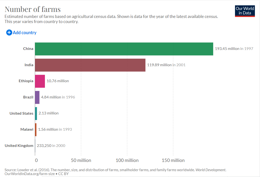
1. I downloaded the Estimated number of farms based on agricultural census data from Our World in Data. I selected this data because I’m interested in seeing how many farms there are and where they’re located.

2. This is the Link to the data.

3. The following code chunk leads the package I will use to read in and prepare the data for analysis.

library(tidyverse)

4. Read the data in

number_of_farms <- read_csv(here::here("_posts/2022-05-10-project-part-1/number-of-farms.csv"))

5. Use glimpse to see the names and types of the columns

glimpse(number_of_farms)

Rows: 111
Columns: 4
$ Entity           <chr> "Albania", "Algeria", "American Samoa", "Ar~
$ Code             <chr> "ALB", "DZA", "ASM", "ARG", "AUS", "AUT", "~
$ Year             <dbl> 1998, 2001, 2003, 1988, 1990, 2000, 1994, 1~
$ all_sizes_number <dbl> 466809, 1023799, 7094, 378357, 129540, 1994~

View(number_of_farms)

6. Use output from glimpse (and View) to prepare the data for analysis.

• create the object ‘countries’ that is a list of countries I want to extract from the dataset

• Change the name of the 1st column to Country and the 4th column to Number of Farms

• Use filter to extract the rows that I want to keep : Year >= 1900 and Country in countries

• Select the columns to keep: Country, Year, Number of Farms

• Use mutate to convert Number of Farms into millions of farms

• Assign the output to country_farms

• Display the first 7 rows of country_farms

Countries <- c( "China",
                "India",
                "Ethiopia",
                "Brazil", 
                "United States",
                "Malawi",
                "United Kingdom")

country_farms <- number_of_farms %>% 
  rename(Country = 1, Farms = 4) %>% 
  filter(Year >=1900, Country %in% Countries) %>% 
  select(Country, Year, Farms) %>% 
  mutate(Farms = Farms * 1e-6)
 
country_farms

# A tibble: 7 x 3
  Country         Year   Farms
  <chr>          <dbl>   <dbl>
1 Brazil          1996   4.84 
2 China           1997 193.   
3 Ethiopia        2002  10.8  
4 India           2001 120.   
5 Malawi          1993   1.56 
6 United Kingdom  2000   0.233
7 United States   2002   2.13 

Check for the total for 2019 equals the total in the graph

country_farms  %>%  filter(Year <= 2006)  %>% 
  summarise(total_emm = sum(Farms))

# A tibble: 1 x 1
  total_emm
      <dbl>
1      333.

Add a picture.

Number of Farms

Write the data to file in the project directory

write_csv(country_farms, file="country_farms.csv")